Houdini
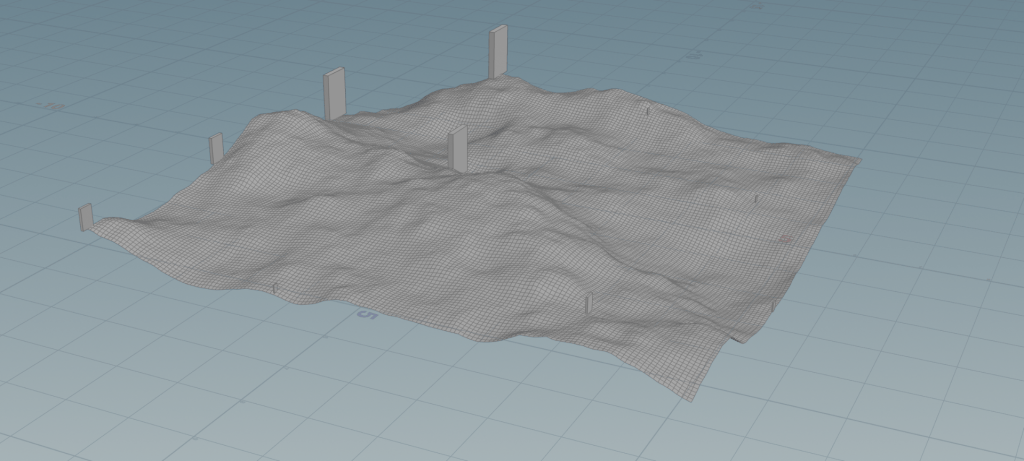
today we spent the first half of the lesson learning the basic commands and steps to take in order to navigate Houdini. We was shown how to transform objects and copy objects, we also dived into creating grids and adding notes to it and playing around with noise and attribute randomizing.
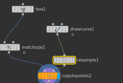
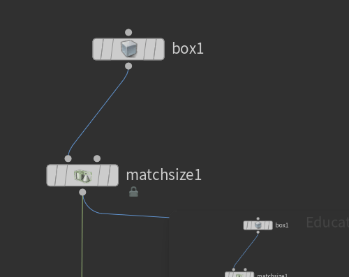
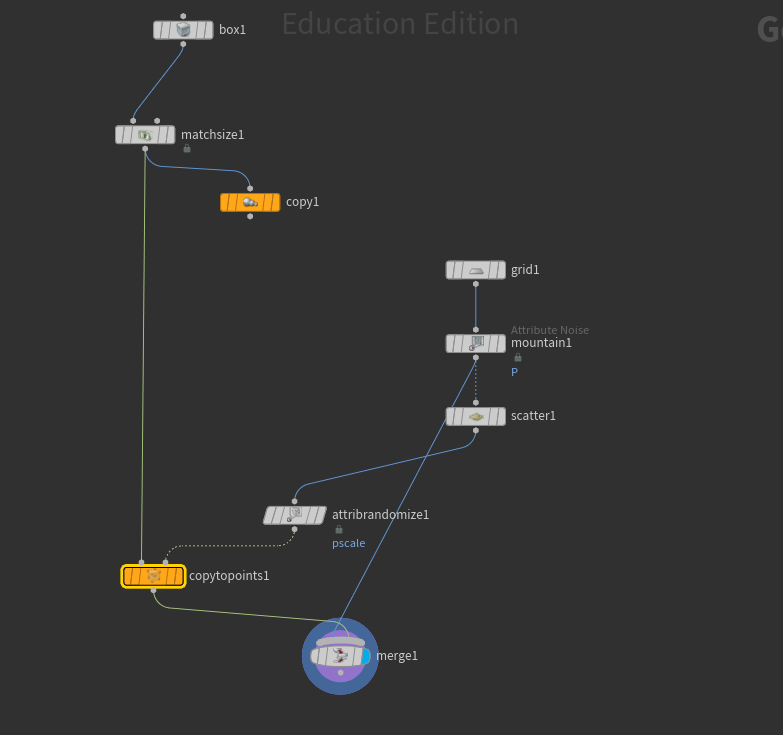
We created dominoes and had them conform to a drawn curve to begin:
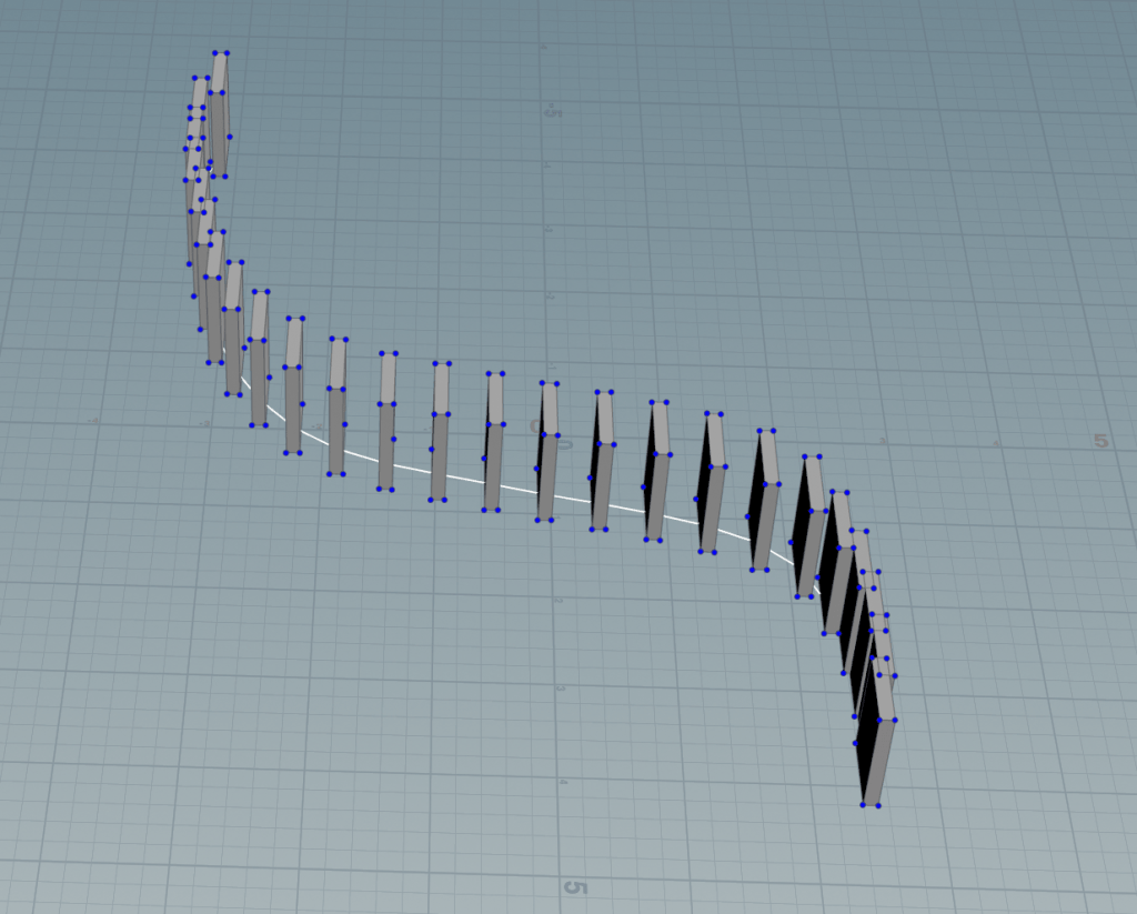
After that we had the dominoes randomised and added a grid below it:
WEEK 2
In todays lessons we retraced our steps of how we built some dominoes, how e drew a curve and done a match size.
Following that we added new nodes such as assemble, point velocity and rbd bullet solver which allow me to
Assembly, manage multiple pieces of geometry with each piece having its own transform and attributes.
Point Velocity, modifies the velocity attribute by points or geometry pieces, I can control movement, wind, explosions pre simulation.
RBD Bullet Solver, calculates collisions, gravity for rigid bodies at high speed.
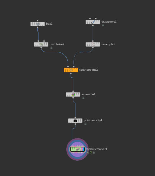
using this node system and the right connections i managed to get to a stage where i could anime the dominios falling over and actually colliding with each other. also a important thing to note is that I MUST add a ground or theyll fall through like my first test.
Ball through wall
Next we started to create a wall and add nodes that would allow fracturing.
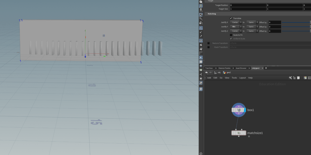
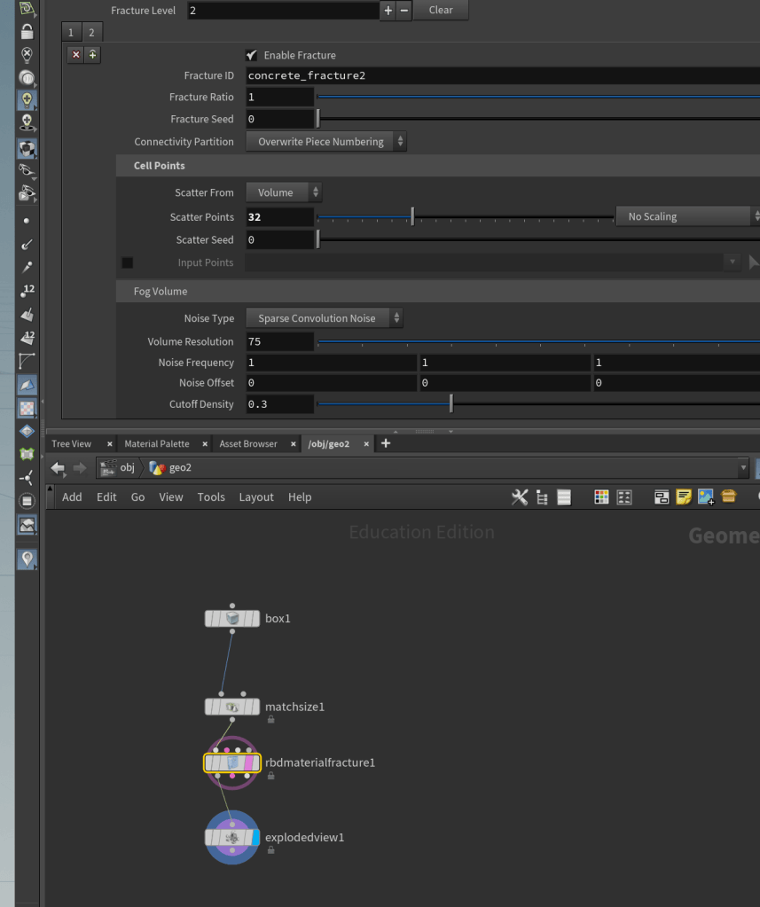
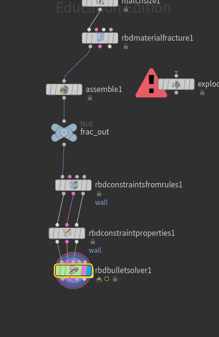
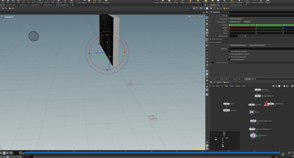
by this stage i had it so that the wall was fractured, when pressing the play button it would automatically crumble so i was then able to add a rbdconstraints that would glue the fractured pieces together. following this i was able to use the slider to choose how strong the bond would be.
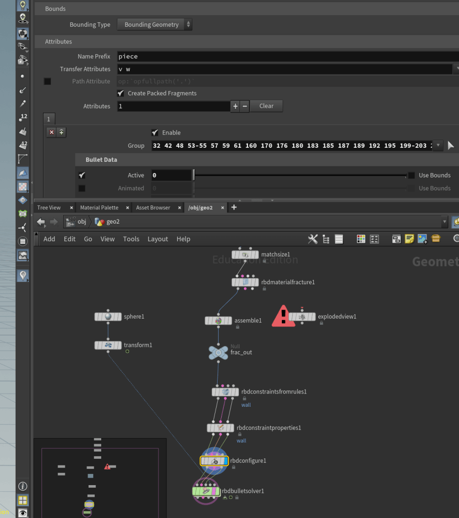
In order to keep the bottom of the wall from moving i added a rbdconfigure which let me choose the bricks i wanted to not move at all.
Above is the finished result of the ball being given a transform. i also had to connect it to the bullet solver and had to hold alt and right location after moving the frames ahead.
STEPS:
- create a wall with matchsize.
- Add rbd material fracture
- change noise type to perlin then i need to adjust scatter in both fracture.
- Add rbd bullet solver, collision and make ground collision.
- Place assemble direcly in the middle of rbd material fracture and rbd bullet solver.
- Add rbd constraint from rules to the rbd bullet solver.
- Add rbd constraints properties to add glue, this acts as a glur to stop the wall breaking. THIS IS BEFORE BULLET SOLVER.
- Connect geometry and proxy geometry and constraint geometry.
- Add a sphere, then using alt + click translate to add a key frame, while moving along the timeline and the balls path into and through the wall.
week 3
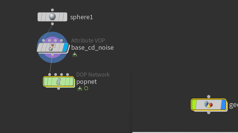
1. I created a geometry and added a sphere. The sphere feeds into an Attribute VOP named base cd noise, then into popnet , setting up the geo for the particle simulation
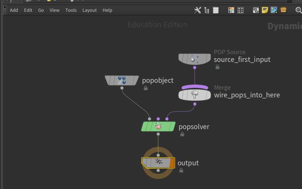
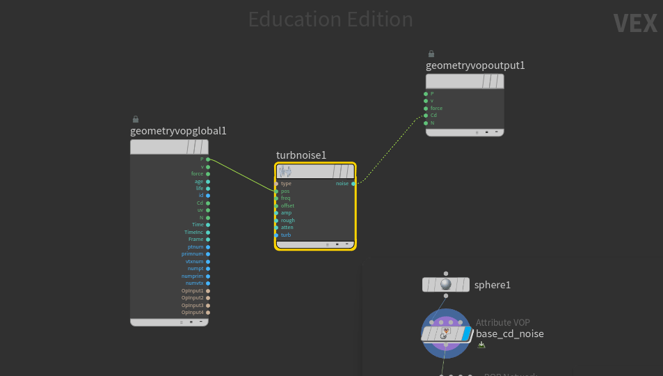
Inside the popnet, the source puts particles into the pop Solver, which updates their motion over time. In the vex network below, a turbulence node modifies the particles’ motion
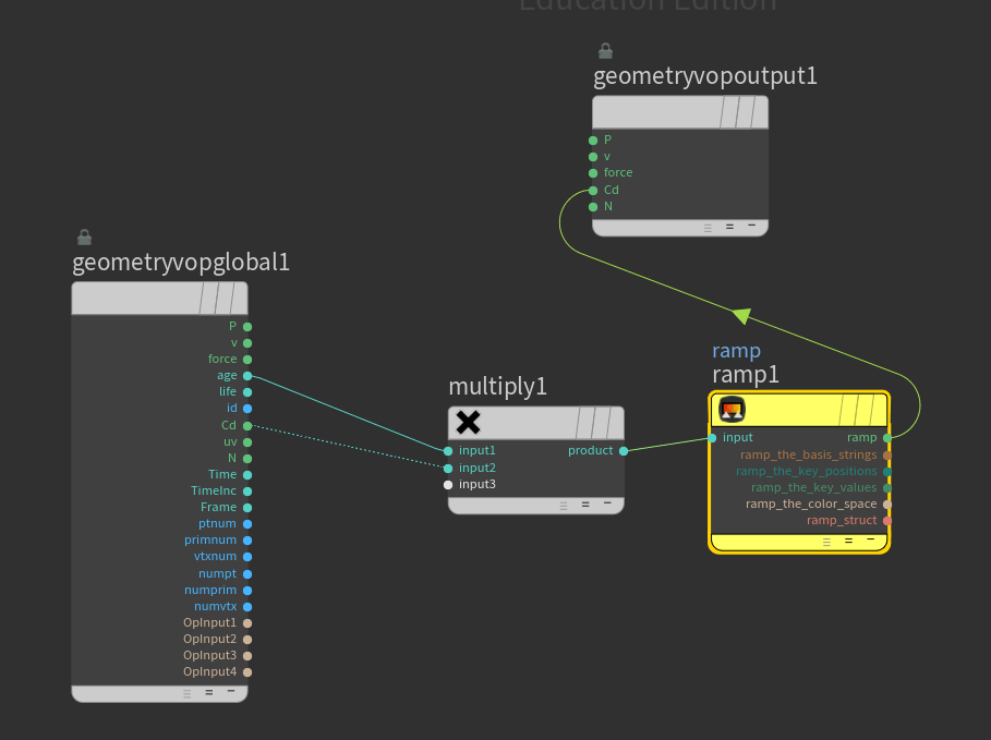
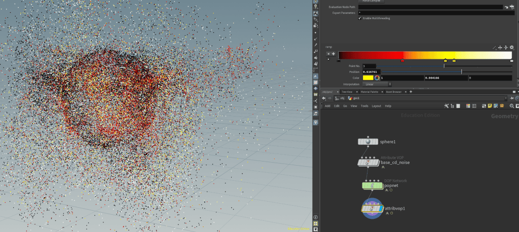
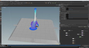
above the particle age is multiplied. the ramp lets me change the colour attribute. in viewport the colors change the cloud of particles with colours red and orange and black and yellow
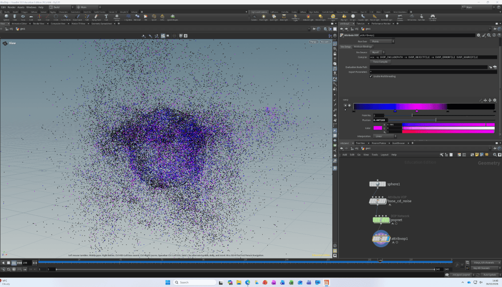
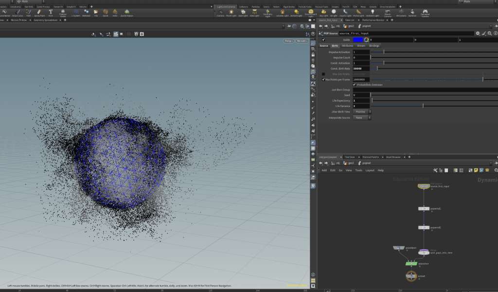
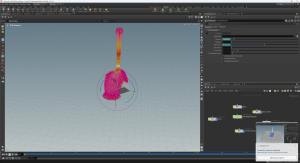
I changed the colour ramp to use purple and blue tones, giving the particle cloud a different colour scheme
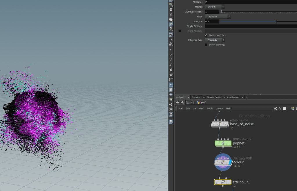
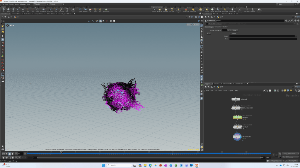
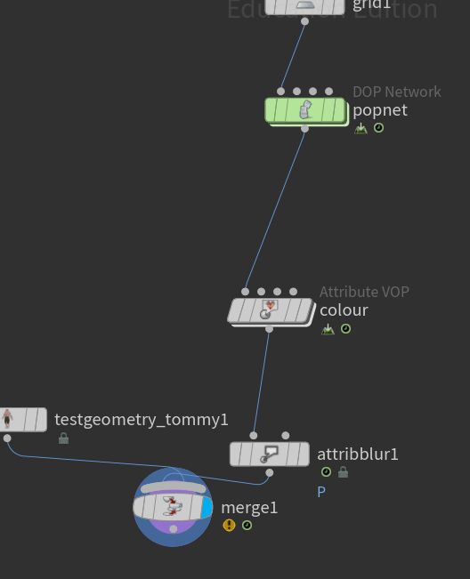
I began with a sphere and used an Attribute VOP to add noise-based colour variation. I then sent the points into a POP simulation, where a POP Solver updates their positions over time. A turbulence node adds irregular motion, causing the point cloud to spread and deform. Particle age is scaled and passed through a colour ramp. the particles’ colour varies with age. I then brought the simulated particles back into the geometry , applied further colour and an Attribute Blur, and viewed the result.
Task 2
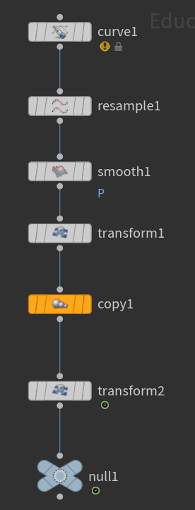
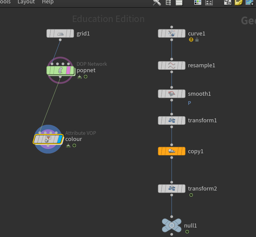
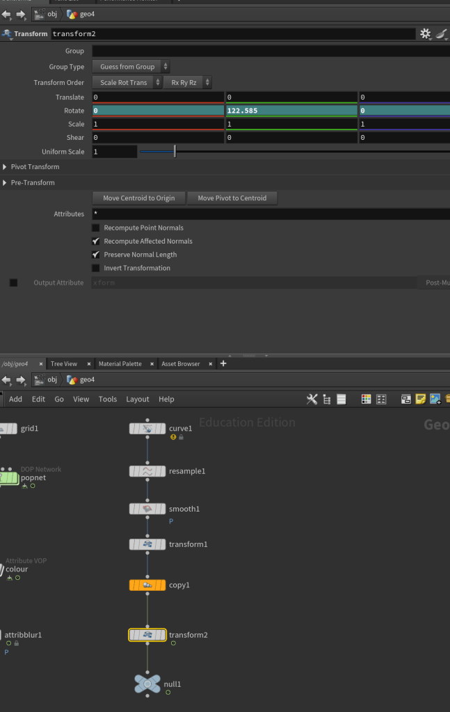
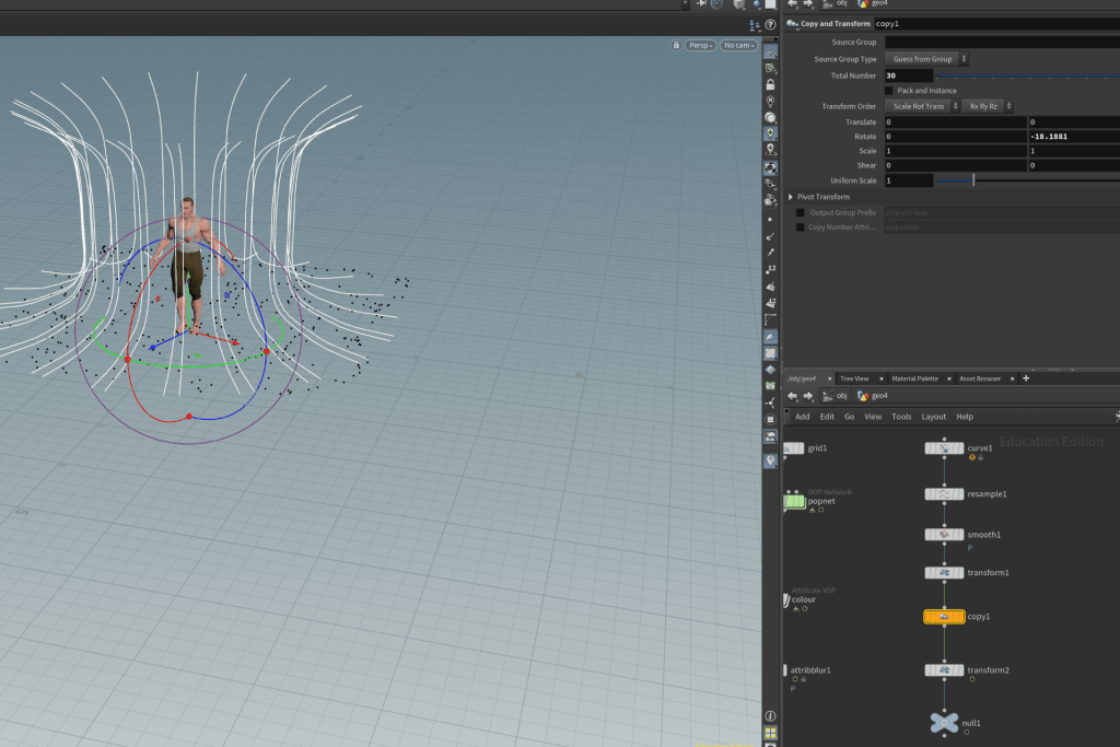
The geometry passes through a Curve node, then Resample, Smooth, and Transform. copy1 node duplicates the geometry. A second Transform adjusts the copies, and the Null node marks the output for the next stage
Step by step
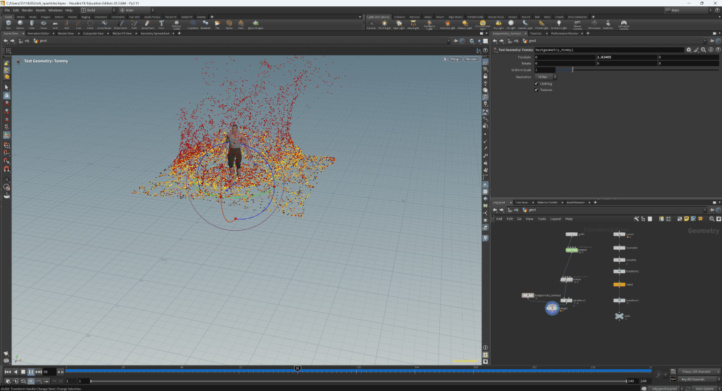
- Grid → POP Network: The grid provides the surface points for a POP simulation.
- Popnet → Attribute VOP: The particles pass through a VOP that sets their colour.
- Curve → Resample: A curve is divided into evenly spaced points, which can be useful as a guide for placing or copying geometry.
- Resample → Smooth: The curve’s point positions are smoothed.
- Smooth → Transform: The processed curve is moved, rotated, or scaled.
- Transform → Copy: The Copy node uses the curve to create repeated geometry.
- Copy → Transform → Null: transform adjusts the copied result and the Null is the end of the geometry chain.
Week 4
WEEK 5